Fourier Transform: Data approximation
From the work of Fourier(1768-1830) we know that every integrable function  defined in
 ![$$[a,b]$](P4Fourier_eq11130704568637826070.png) can be approximate by a sum of trigonometric functions:
can be approximate by a sum of trigonometric functions:
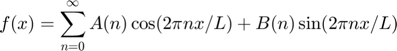 .
.
Here  and because Fourier transform is specilly appropiate for periodic functions we can make a change of variables in the x variables a get the expressions for the Fourier coefficients as
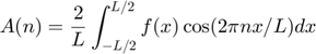
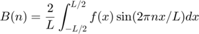
and analogously
Compact representation:
If we define Phases as 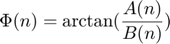 and amplitudes as
  , Fourier transform can be also written as
 .
.
Contents
- A Simple Example:
- Compute Discrete Fourier Transform
- Compute Inverse Fourier Transform
- Frequencies and Magnitudes
- General Data Approach: Function through a data set.
- General Data Using Fast Fourier Transform from Matlab
- Fourier transform analysis
- Numerical trigonometric interpolation in a new point
- Discrete Fourier Transform Function
- Inverse Fourier Transform Function
- (c) Numerical Factory 2019
A Simple Example:
Consider one funcion  defined on
 ![$$[0,2\pi]$](P4Fourier_eq04024897143965832866.png) and we evaluate on
and we evaluate on  where
where  is the number of subdivisions.
clear all;
close all;
Ndiv=8;
h=2*pi/Ndiv;
x=0:h:2*pi-h; %don't take last point (it is supposed to be the same as 0)
f=sin(x)+cos(x);

N=length(f);
Compute Discrete Fourier Transform
For N values we consider the points in the interval [-N/2, N/2] (this is more stable from a numerical point of view) and we approximate the integral by the sumatory (trapezoidal's rule).
By deffault we compute as many Fourier coefficients than number of points.
for k=0:N-1
    sumA=0;
    sumB=0;
    for j=0:N-1
        sumA=sumA+f(j+1)*cos(2*pi*j*(k-N/2)/N);
        sumB=sumB+f(j+1)*sin(2*pi*j*(k-N/2)/N);
    end
    A(k+1)=sumA/N;
    B(k+1)=sumB/N;
end
Compute Inverse Fourier Transform
Once we have the Fourier coefficients we can use the Fourier series to approximate the true value f at each point.
We increase the order approximation to visualize convergence of the sumatory. Notice that only 3 coefficients are enought for this particular function
for order=1:N-1
    plot(x,f,'o-'); %plot the original function
    hold on;
    for k=0:N-1
        sum=0;
        for j=0:order
            sum=sum+A(j+1)*cos(2*pi*k*(j-N/2)/N)+B(j+1)*sin(2*pi*k*(j-N/2)/N);
        end
        faprox(k+1)=sum;
    end
    plot(x,faprox,'*-'); %plot the approximated points
    Error(order)=max(abs(f-faprox));
end
hold off;
disp('Error at each order approximation');
Error'
Error at each order approximation

ans =

    1.4142
    1.4142
    0.7071
    0.7071
    0.0000
    0.0000
    0.0000

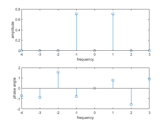
Frequencies and Magnitudes
We can represent the frequences space and the associated magnitudes from the previous formulas
for i=1:N
    Atilde(i)=sqrt(A(i)^2+B(i)^2);
    Phi(i)=atan(B(i)/A(i));
end
figure()
subplot(2,1,1)
    stem(-N/2:N/2-1,Atilde)
    xlabel('frequency');ylabel('amplitude')
subplot(2,1,2)
    stem(-N/2:N/2-1,Phi)
    xlabel('frequency');ylabel('phase angle')
General Data Approach: Function through a data set.
Consider now that you have a set of measure data and you want to compute a function passing through these data. The Fourier approximation allow us to compute this function.
We will define (at the bottom of this document) the two functions:
- Discrete Fourier Transform: function fcoeff=DiscFourierTrans(f,N)
- Inverse Fourier Transform: function faprox=invFourierTrans(fcoeff,N,order)
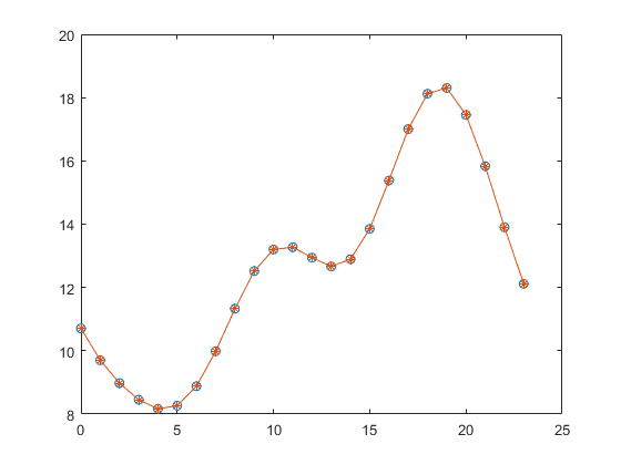
%Consider a set of data values
f=[10.7083
    9.7003
    8.9780
    8.4531
    8.1653
    8.2633
    8.8795
    9.9850
   11.3289
   12.5172
   13.2012
   13.2720
   12.9435
   12.6647
   12.8940
   13.8516
   15.3819
   17.0033
   18.1227
   18.3039
   17.4531
   15.8322
   13.9056
   12.1154];
x=0:length(f)-1; % here x is just the enumeration of the data values.
N=length(x);
fcoeff=DiscFourierTrans(f,N);
order=15; %try order = 13, 14 to see the different approximation
faprox=invFourierTrans(fcoeff,N,order);
figure()
plot(x,f,'o-'); %plot the approximated points
hold on;
plot(x,faprox,'*-'); %plot the approximated points
General Data Using Fast Fourier Transform from Matlab
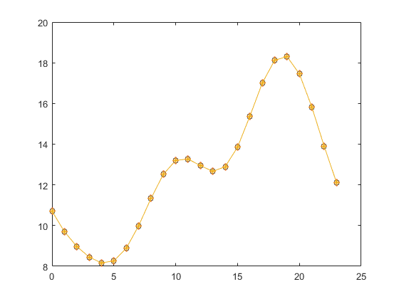
We solve the same previous example but using now Matlab function Fast Fourier Transform (fft)
Fourier transform analysis
P1 = fft(f)/N; %fast Fourier transform
P2=fftshift(P1);
% You can recover the real coefficients
    fcoeff=[real(P2),-imag(P2)];
    order=15;
    faprox=invFourierTrans(fcoeff,N,order); %using our function
% or you can use the compact Fourier formula
    amp=abs(P2); % amplitude for complex variables
    phi = angle(P2); % phase angle for complex variables
    for k=0:N-1
        sum=0;
        for j=0:order
            sum=sum+amp(j+1)*cos(2*pi*k*(j-N/2)/N+phi(j+1));
        end
        faproxCompact(k+1)=sum;
    end


figure()
title('Now using fft')
plot(x,f,'s-'); %plot the approximated points
hold on;
plot(x,faprox,'d-'); %plot the approximated points
plot(x,faproxCompact,'*-'); %plot the approximated points
Numerical trigonometric interpolation in a new point
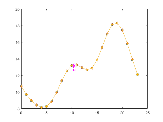
Once we have the Fourier approximation of a set of data, we can use it to approximate the corresponding value for an unknown point not belonging to the data set.
We can use different order approximation and see how the new value behaves. Below we show for the point 10.5 (not in the original table) how the approximations of different Fourier order fits the original interpolated curve. For the maximum order (15) the interpolated value is on the curve.
point=10.5;
order=[12,13,15];
for i=1:3
    sum=0;
    for j=0:order(i)
        sum=sum+amp(j+1)*cos(2*pi*point*(j-N/2)/N+phi(j+1));
    end
    fvalue(i)=sum;
end
xx=point*ones(3,1); % just to plot
plot(xx,fvalue','sm'); %plot the approximated points
Discrete Fourier Transform Function
function fcoeff=DiscFourierTrans(f,N)
    for k=0:N-1
        sumA=0;
        sumB=0;
        for j=0:N-1
            sumA=sumA+f(j+1)*cos(2*pi*j*(k-N/2)/N);
            sumB=sumB+f(j+1)*sin(2*pi*j*(k-N/2)/N);
        end
        A(k+1)=sumA/N;
        B(k+1)=sumB/N;
    end
    fcoeff=[A;B]';
end
Inverse Fourier Transform Function
function faprox=invFourierTrans(fcoeff,N,order)
    if (order >=N), order=N-1; end;
    A=fcoeff(:,1);
    B=fcoeff(:,2);
    for k=0:N-1
        sum=0;
        for j=0:order
            sum=sum+A(j+1)*cos(2*pi*k*(j-N/2)/N)+B(j+1)*sin(2*pi*k*(j-N/2)/N);
        end
        faprox(k+1)=sum;
    end
end
(c) Numerical Factory 2019
(see this video for more intuition https://www.youtube.com/watch?reload=9&v=spUNpyF58BY )