1D Model Equation: Error according to the Finite Element Solution
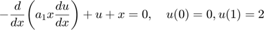
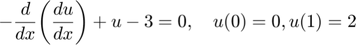
Consider the following problem
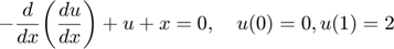
or using the usual ODE notation:

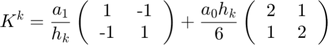
It correspond to the model equation with 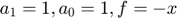 . For each element
 ![$$\Omega^k=[x_i,x_{i+1}]$](Fem1DPractError_eq02467726294318238257.png) we get a (constant coefficients) part and a variable one that we can express as
we get a (constant coefficients) part and a variable one that we can express as
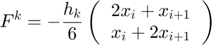
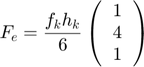
and from the variable f(x)=-x (on the right hand side), for each element we have
We will assembly the global system ![$$[K]u = F + Q$](Fem1DPractError_eq00871387503019692773.png) , according to the element decomposition and Boundary Conditions
, according to the element decomposition and Boundary Conditions
Compute the FEM1D numerical results for  and give the error

(Hint: in Matlab  is written as norm(v,inf))
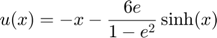
with respect to the actual solution
Contents
Geometry
The column is divided in numDiv equal elements of length h.
clear all;
fout=fopen('ErrorAprox.txt','w');
fprintf(fout,' NunELem      h        Error \n');
solution=@(x) -x-(6*exp(1)/(1-exp(1)^2))*sinh(x);
L=1; a1=1; a0=1;
numDiv=[5,50,500,5000];
results=[];
for iter=1:length(numDiv)
    numElem=numDiv(iter);
    clear K;
    h=L/numElem;
    nodes=(0:h:L)'; %colum vector
    for i=1:numElem
           elem(i,:)=[i, i+1];
    end
    numNod = size(nodes,1);
    numElem = size(elem,1);
Assembly of the Global System
    Ke=a1/h*[1,-1;-1,1]+a0*h/6*[2,1;1,2]; %local stiff matrix (constant!!)
    K = zeros(numNod); %initialize the global Stiff Matrix
    F = zeros(numNod,1); %initialize the internal forces global vector
    Q = zeros(numNod,1); %initialize the global Q vector
    for i=1:numElem
           rows=[elem(i,1); elem(i,2)];
           colums= rows;
           K(rows,colums)=K(rows,colums)+Ke; %assembly Stiff matrix
           % Assembly of the  non-constant F terms
           nod1 = elem(i,1);
           nod2 = elem(i,2);
           Fe=[-h/6*(2*nodes(nod1)+nodes(nod2));-h/6*(nodes(nod1)+2*nodes(nod2))];
           F(rows,1)=F(rows,1)+Fe;
    end
    Fini=F; %copy the original F values for the postprocess
Boundary Conditions
    fixedNodes=[1,numNod]; %Fixed Nodes (global num.)
    freeNodes = setdiff(1:numNod,fixedNodes); %Complementary of fixed nodes
    % modify the linear system, here BC are NOT 0.
    u=zeros(numNod,1); %initialize u vector
    u(1)=0; %BC at x=0
    u(numNod)=2; %BC at x=1
    Q=Q-K(:,fixedNodes)*u(fixedNodes);
    %-u(1)*K(:,1)-u(numNod)*K(:,numNod);

    Km=K(freeNodes,freeNodes);
    Fm=F(freeNodes)+Q(freeNodes);
    % solve the System
    format short e; %just to a better view of the numbers
    um=Km\Fm;
    u(freeNodes)=um;

    % Post process
    Q=K*u-Fini;

    %%-----Chek errors
    x=nodes; %for 1D problems coord are the only value in nodes
    ureal=solution(x);
    error=norm(u-ureal,inf);
    fprintf(fout,'%4d     %e  %e \n', numElem, h, error);
end
fclose(fout);
type('ErrorAprox.txt'); %show file in Matlab editor
 NunELem      h        Error
   5     2.000000e-01  5.331016e-04
  50     2.000000e-02  5.304443e-06
 500     2.000000e-03  5.306718e-08
5000     2.000000e-04  7.449230e-10
Excercise 1: Non-constant coefficient a1 (linear)
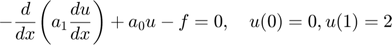
Modify this matlab code in order to solve also the non-constant case coefficient  (linear). The equation can stated as
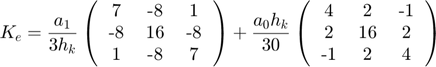
where the element stiffness matrix has the expression (see the first problem on the class list exercices):
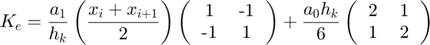
Find the mean value of the solution when only 10 equal linear elements are considered and a1=1. Notice that now it is not possible to compare with a true solution.
Sol: 1.140151e+00
Exercise 2: Constant 1D quadratic elements
Modify this matlab code in order to solve the constant problem with quadratic elements.
The equation can stated as:
where the element stiffness matrix has the expression (see the fourth problem on the class list exercices):
Solve the following differential equation using 4 quadratic elements and compute the mean solution:
Hint: Here you have to addapt the mesh (nodes and elements) using
h=L/numElem;
nodes=(0:0.5*h:L)'; %colum vector
for i=1:numElem
      k=1+2*(i-1);
      elem(i,:)=[k, k+1, k+2];
end
and also the assembly for loop using 3 nodes for each row.
Sol: 1.132557e+00
(c)Numerical Factory 2019