Gauss1D

1D Gaussian Quadratures
Function to integrate
Order of integration (number of Gauss points)
The final formula
Exercise 1:
Exercise 2:

1D Gaussian Quadratures

We will implement a function that give us the associated Gauss quadrature points and their weigths.

We will apply this to the computation of the integral of a polynomial funcion (exact) and general functions (approximate).

$$\int{f(x) dx}= \sum \omega_i f(pG_i)$

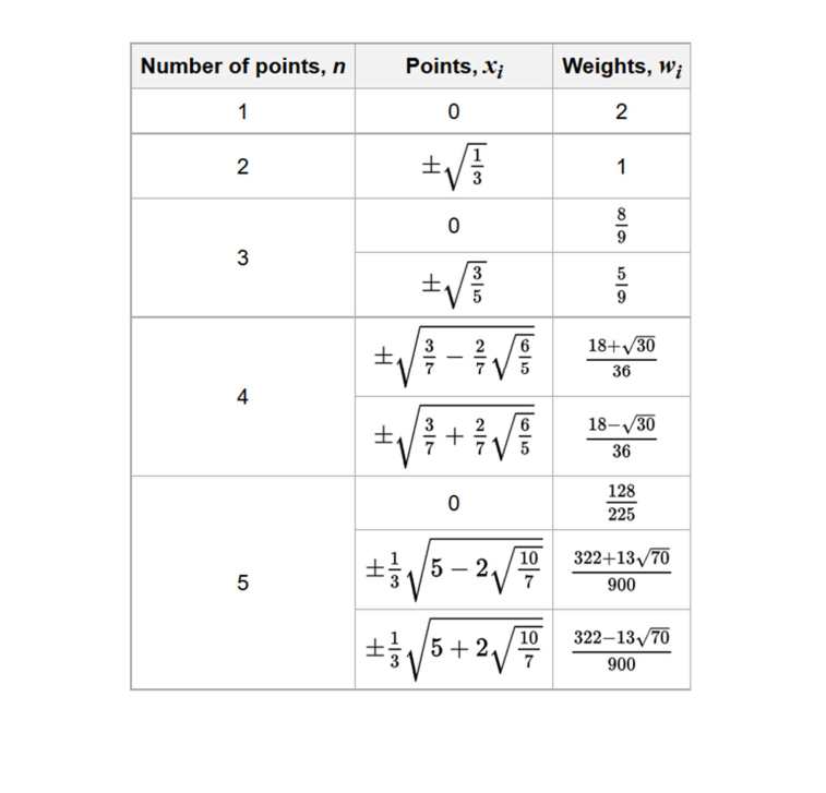
imagePlot('GaussTable.png',100);

Function to integrate

Let's consider the function

$$ f(x)=x^4-3x^2+1$

f=@(x) x.^4-3*x.^2+1; %defined as inline function

or as a file function

function y=f(x)

y=x.^4-3*x.^2+1;

Order of integration (number of Gauss points)

As you increment n the formula is exact for polynomials of degree 2n-1.

n=3;
switch (n)
    case 1
        w=2; pG=0;
    case 2
        w=[1,1]; pG=[-1/sqrt(3), 1/sqrt(3)];
    case 3
        w=[5/9, 8/9, 5/9]; pG=[-sqrt(3/5), 0, sqrt(3/5)];
    otherwise
        error('No data are defined for this value');
end

The final formula

You can use a sequential formula

sumat = 0;
for i=1:size(pG,2)
    sumat = sumat + w(i)*f(pG(i));
end
intFseq = sumat

intFseq =

    0.4000

or equivalently, a compact form of the same value

intFcompact = sum(w.*f(pG))

intFcompact =

    0.4000

Check the error against the actual value

primitiveF=@(x) x.^5/5-x.^3+x;
barrowRule=primitiveF(1)-primitiveF(-1);
errorInt = abs(barrowRule - intFcompact)

errorInt =

   2.2204e-16

Exercise 1:

make the assignment of the Gauss points and weight values a Matlab function for n=1,..5 (check n <=5, bigger values are not allow, use the following sentence).

error('No data are defined for this value');

According to the table included above you have to implement and get the results:

function [w,pt] = gaussValues1D(n)

imagePlot('GaussTable.png',100);
for n=1:6 %for n=6 must return an error
    n
    [w,pt]=gaussValues1D(n) %function to be implemented
end

n =

     1


w =

     2


pt =

     0


n =

     2


w =

     1     1


pt =

   -0.5774    0.5774


n =

     3


w =

    0.5556    0.8889    0.5556


pt =

   -0.7746         0    0.7746


n =

     4


w =

    0.6521    0.6521    0.3479    0.3479


pt =

   -0.3400    0.3400   -0.8611    0.8611


n =

     5


w =

    0.4786    0.4786    0.5689    0.2369    0.2369


pt =

   -0.5385    0.5385         0   -0.9062    0.9062


n =

     6

Error using gaussValues1D (line 19)
No data are defined for this value

Error in Gauss1D (line 71)
    [w,pt]=gaussValues1D(n) %function to be implemented

Exercise 2:

Using the function gaussValues1D, approximate the value of the integral in [-1,1] of the function f(x)=cos(x). Use different values of n and show the errors comparing with the true value 2*sin(1)

Sol:

n, error

1   3.1706e-01

2   7.1183e-03

3   6.1578e-05

4   2.8092e-07

5   7.9140e-10