PostProcess: using color with Matlab plots

Contents

Show results using color values

Matlab allow us to plot the results on the nodes of one element using color interpolation. The main function is FILL.

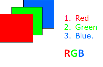
Color in general is defined as a triplet RGB values [r,g,b]

red: 0 <= r <= 255 (integer) or 0.0 <= r <= 1.0 (float) is the first channel [r,0,0]

green: 0 <= g <= 255 (integer) or 0.0 <= g <= 1.0 (float) is the second channel [0,g,0]

blue: 0 <= b <= 255 (integer) or 0.0 <= b <= 1.0 (float) is the third channel [0,0,b]

Color in Matlab can be specified using RGB but it also uses colormap which is an array of colors according to certain rules (jet, gray, copper, etc.) (see doc colormap in Matlab for more information)

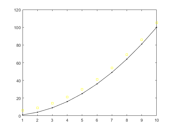
x=1:10;
y=x.^2;
plot(x,y,'.-','Color',[0.0,0.0,0.0]) %black color
hold on;
plot(x,y+5,'s','Color',[1.0,1.0,0.0]) %yelow color
hold off;

Colormap

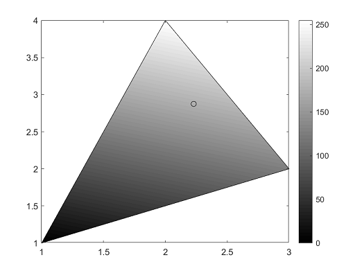
When only one value is associated to each point, Matlab offers the possibility of chossing a color scale named colormap ( jet by default). It consist of a table of 64 RGB different colors associated from the maximum value (red) to the minimum one (blue).

Let's see an exemple considering only one element: We consider a simple example where a Triangle is defined by its nodes and a numerical value is associated to each node.

Using the FILL function a color representation is obtained where each point on the triangle has an interpolated color computed from the vertices values and the colormap.

nodes=[1,1;  %define the nodes of a triangle
    3,2;
    2,4];
elem=[1,2,3]; %define the triangle it self as an element
X=nodes(:,1);
Y=nodes(:,2);
values=[0;128;255]; %can be temperature, stress, etc.
fill(X,Y,values);
colormap('jet') %one of the standar color maps for FEM
colorbar %it is optional, shows the bar with the color scale
hold on;
p=[2,3]; %consider a point
plot(p(1,1),p(1,2),'ko'); %plot the point using a black o
hold off;

Exercise 1:

Use the same value for all nodes and you will get a flat color triangle

Use also colormap('gray') to obtain a gray color image

A color triangle mesh

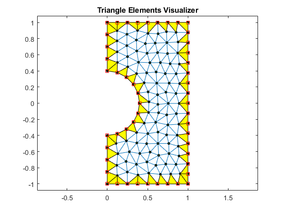
Using the previous approach one can represent the color interpolation of each triangle in a triangle mesh.

We have build a general function plotContourSolution.m in this case.

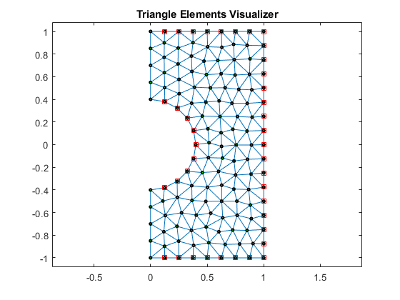
Consider the triangle mesh in meshHole.m and assign a value of temperature for each node (like in one of our previous practices).

eval('meshHole');
numNodes=size(nodes,1);
numElem=size(elem,1);

% Just as an example we gave a temperature value for each node
Temp=1:numNodes; %temperature for node i is assigned as T(i)=i;

titol='Temperature Plot';
colorScale='jet';
% We will use our own function for plotting a colored mesh
% it can plot both triangular and quadrangular meshes.
plotContourSolution(nodes,elem,Temp,titol,colorScale);

Exercise 2:

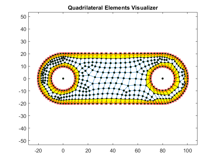
Plot the quadrangular mesh meshTwoHolesQuad.m using the above function.

Selection of a set of points: Boundaries

From the nodes of a mesh, we can select different set of points from a mathematical equation or condition.

The Matlab function to use is find. It allow us to recover the indices (row and column) of a table that meets a condition. The sintax is:

[indRow, indCol]= find(condition)

Example: Select the left boundary nodes according their x-coordinate. Instead of using =0, we introduce a small tolerance (better when using floats)

[indexLeft, indCol]=find(nodes(:,1)<0.01); %index are the node numbers
hold on;
plot(nodes(indexLeft,1),nodes(indexLeft,2),'mo')

Exercise 3:

Compute the index set for all points in the boundary of the meshHole example. Make different selection for the left, rigth, top, botton and circle segment boundaries and build an indexBoundary vector using all of them. You must obtain the following number of nodes:

indexLeft: 10, indexRight:17, indexTop: 9, indexBottom: 9, indexCircle: 11

indexBoundary: 50

Hint. Use the Matlab function unique to erase repeated nodes in the global indexBoundary vector.

Recovering all boundary points

We have also a function to obtain all the boundary nodes and elements.

[indNodBd, indElemBd, indLocalEdgBd, edges] = boundaryNodes(nodes, elem);
fprintf(' number of Boundary nodes = %d \n',length(indNodBd));
fprintf(' number of Boundary elements = %d \n',length(indElemBd));

% show the elements and nodes at the boundary
figure()
plotElements(nodes, elem, 0);
hold on;
for i=1:length(indElemBd)
    fill(nodes(elem(indElemBd(i),:),1),nodes(elem(indElemBd(i),:),2),'y')
end
plot(nodes(indNodBd,1), nodes(indNodBd,2),'rs');
hold off;

%
% You can substract some of the boundary node sets
% using the *setdiff* Matlab function
%
newNodesBd=setdiff(indNodBd,indexLeft);
figure()
plotElements(nodes, elem, 0);
hold on;
plot(nodes(newNodesBd,1), nodes(newNodesBd,2),'rs');
hold off;

 number of Boundary nodes = 50 
 number of Boundary elements = 50 

Exercise 4:

Compute the number of nodes in the boundary of the meshTwoHolesQuad.m example. using the boundaryNodes function.

Sol= 170

% *(c)Numerical Factory 2019*

Published with MATLAB® R2018a