FEM2D: Thermal convection problems using Triangular Elements

Consider the 2D equation model, a second order PDE equation with general coefficients a11, a12, a21, a22, a00, f :

Contents

Engine cooling fin: State the problem

Consider the mesh file meshAleta2DTriang.m which represents half of the geometry of the cooling fin shown at the figure with the Bondary Conditions stated there.

Take the material conductivity coefficient kc=0.5 and no internal heat source (f=0).

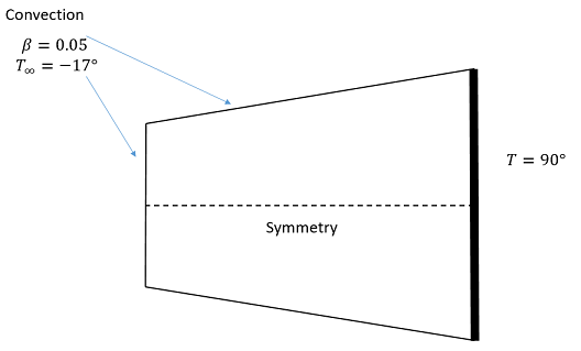
Question: Find the temperature at the point P=[0.9,2.1].

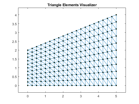
Define Geometry: node coordinates and elements

eval('meshAleta2DTriang');
numNod=size(nodes,1);
numElem=size(elem,1);
numbering=0;
plotElements(nodes,elem,numbering);

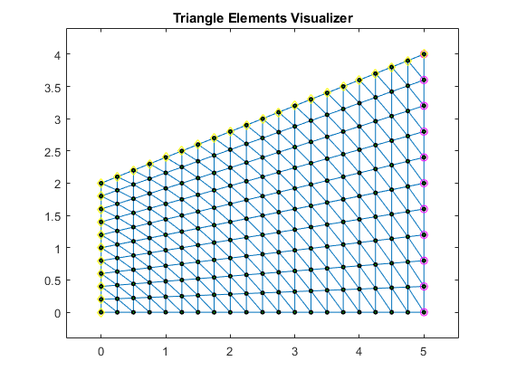
Select Boundary points

indLeft=find(nodes(:,1) < 0.01);
indRight=find(nodes(:,1) > 4.99);
indTop=find(abs(2*nodes(:,1)/5 +2 - nodes(:,2))< 0.01);
hold on;
plot(nodes(indLeft,1),nodes(indLeft,2),'yd');
plot(nodes(indRight,1),nodes(indRight,2),'mo');
plot(nodes(indTop,1),nodes(indTop,2),'yd');
hold off;

Define Coefficients vector of the model equation

In this case we use the Poisson coefficients defined in the problem above

a11=0.5;
a12=0;
a21=a12;
a22=a11;
a00=0;
f=0;
coeff=[a11,a12,a21,a22,a00,f];

Compute the global stiff matrix

Use the linearTriangElement function to compute the system by element

K=zeros(numNod);   %global Stiff Matrix
F=zeros(numNod,1); %global internal forces vector
Q=zeros(numNod,1); %global secondary variables vector
for e=1:numElem
  % compute element system
    [Ke,Fe]=linearTriangElement(coeff,nodes,elem,e);
  %
  % Assemble the elements
  %
    rows=[elem(e,1); elem(e,2); elem(e,3)];
    colums= rows;
    K(rows,colums)=K(rows,colums)+Ke; %assembly
    if (coeff(6) ~= 0)
        F(rows)=F(rows)+Fe;
    end
end % end for elements
% make a copy of the original matrices
Korig = K;
Forig = F;

Boundary Conditions (BC)

Impose Boundary Conditions for this example. In this case only essential and natural BC are considered. We will do a thermal example for convection BC (mixed).

fixedNodes=[indRight']; %Fixed Nodes (global num.)
freeNodes = setdiff(1:numNod,fixedNodes); %Complementary of fixed nodes

% ------------ Convection BC
convecNodes=[indLeft', indTop']; %must be a row vector
convecNodes=unique(convecNodes); %to avoid duplicate nodes
beta=0.05; %Convection Coefficient
Tinf=-17; %Bulk temperature
[K,Q]=applyConvTriang(convecNodes,beta,Tinf,K,Q,nodes,elem);

% ------------ Essential BC
u=zeros(numNod,1); %initialize u vector
u(indRight)=90; %all of them are zero
F=F-K(:,fixedNodes)*u(fixedNodes);%here u can be different from zero only for fixed nodes

% modify the linear system.
Km=K(freeNodes,freeNodes);
Im=F(freeNodes)+Q(freeNodes);

Compute the solution

solve the System

format short e; %just to a better view of the numbers
um=Km\Im;
u(freeNodes)=um;

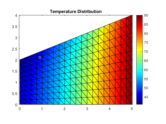
PostProcess: Compute secondary variables and plot results

titol='Temperature Distribution';
colorScale='jet';
plotContourSolution(nodes,elem,u,titol,colorScale);

p=[0.9,2.1];
hold on;
plot(p(1),p(2),'ys');
hold off;
for i=1:numElem
    v1=nodes(elem(i,1),:);
    v2=nodes(elem(i,2),:);
    v3=nodes(elem(i,3),:);
    vertices=[v1; v2; v3];
    [alphas, isInside]=baryCoord(vertices, p);
    if (isInside == 1)
        ntri=i;
        break;
    end
end
% interpolate temperature
temp=alphas*u(elem(ntri,:))

temp =

   4.6757e+01

(c)Numerical Factory 2019

Published with MATLAB® R2017b