FEM2D: Thermal problem using Triangular Elements

Consider the 2D equation model, a second order PDE equation with general coefficients a11, a12, a21, a22, a00, f :

Contents

Equations for Thermal problems

Assume the case and .

State the problem:

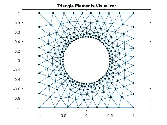
Consider an square domain [-1,1]x[-1,1] with a circular hole in the middle (CircleHoleMesh01.m)

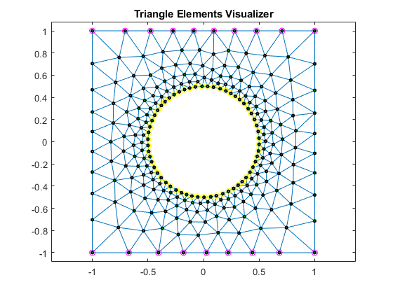
As a BC, consider the circle points at 50ºC and top and bottom boundaries at 10ºC.

Load Geometry: node coordinates and elements

clear all;
eval('CircleHolemesh01');
numNod=size(nodes,1)
numElem=size(elem,1)
numbering=0; %=1 shows nodes and element numbering
plotElements(nodes,elem,numbering);

numNod =

   260


numElem =

   427

Select Boundary points

indTop=find(nodes(:,2)> 0.99);
indBot=find(nodes(:,2)< -0.99);
indCircle=find(sqrt(nodes(:,1).^2+nodes(:,2).^2)<0.501);
hold on;
plot(nodes(indTop,1),nodes(indTop,2),'mo');
plot(nodes(indBot,1),nodes(indBot,2),'mo');
plot(nodes(indCircle,1),nodes(indCircle,2),'yo');
hold off;

Define Coefficients vector of the model equation

In this case we use the Poisson coefficients defined in the problem above

a11=1;
a12=0;
a21=a12;
a22=a11;
a00=0;
f=0;
coeff=[a11,a12,a21,a22,a00,f];

Compute the global stiff matrix

Use the linearTriangElement function to compute the system by element

K=zeros(numNod);   %global Stiff Matrix
F=zeros(numNod,1); %global internal forces vector
Q=zeros(numNod,1); %global secondary variables vector
for e=1:numElem
  % compute element system
    [Ke,Fe]=linearTriangElement(coeff,nodes,elem,e);
  %
  % Assemble the elements
  %
    rows=[elem(e,1); elem(e,2); elem(e,3)];
    colums= rows;
    K(rows,colums)=K(rows,colums)+Ke; %assembly
    if (coeff(6) ~= 0)
        F(rows)=F(rows)+Fe;
    end
end % end for elements
% we save a copy of the initial F array
% for the postprocess step
Fini=F;

Boundary Conditions (BC)

Impose Boundary Conditions for this example. In this case only essential and natural BC are considered. We will do a thermal example for convection BC (mixed).

fixedNodes=[indTop', indBot', indCircle']; %Fixed Nodes (global num.)
freeNodes = setdiff(1:numNod,fixedNodes); %Complementary of fixed nodes
% ------------ Essential BC
u=zeros(numNod,1); %initialize u vector
u(indTop)=10; %all of them are zero
u(indBot)=10; %all of them are zero
u(indCircle)=50; %all of them are zero
F=F-K(:,fixedNodes)*u(fixedNodes);%here u can be different from zero only for fixed nodes
% ------------ Natural BC
Q(freeNodes)=0; %all of them are zero
% modify the linear system, this is only valid if BC = 0.
Km=K(freeNodes,freeNodes);
Im=F(freeNodes)+Q(freeNodes);

Compute the solution

solve the System

format short e; %just to a better view of the numbers
um=Km\Im;
u(freeNodes)=um;
%u(fixedNodes)=0;

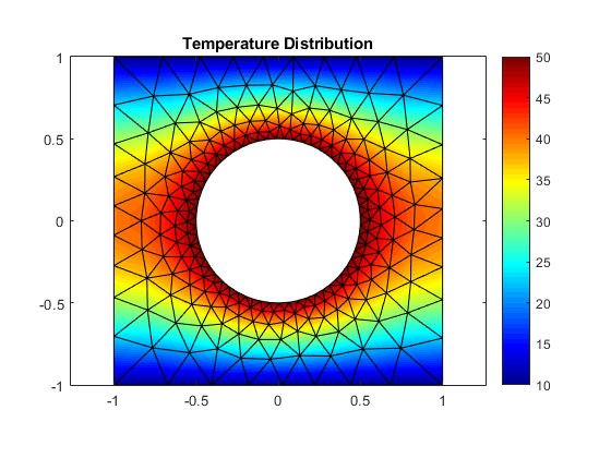
PostProcess: Compute secondary variables and plot results

Q=K*u-Fini;
titol='Temperature Distribution';
colorScale='jet';
plotContourSolution(nodes,elem,u,titol,colorScale);

Exercise 1:

Compute the temperature for the point p=[0.5, 0.8].

Sol: pElem = 206, nodes=[172, 221, 177], tempP = 2.1258e+01

(c)Numerical Factory 2017

Published with MATLAB® R2017b