FEM2D: Thermal problem with Convection BC using Triangular Elements

Equations for Thermal problems Assume the case $$k_c=1$ and $$f=0$ .

State the problem:
Define Geometry: node coordinates and elements
Define Coefficients vector of the model equation
Compute the global stiff matrix
Boundary Conditions (BC)
Compute the solution
Post Process
Apply Convection Boundary Conditions on a Triangle mesh

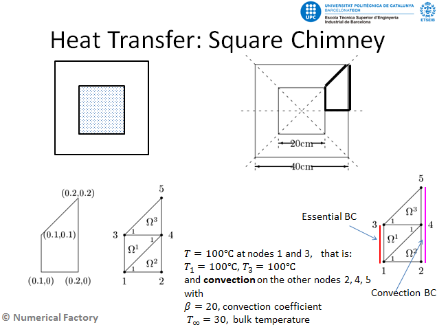
State the problem:

Consider a square Chimney 40x40 cm with a square hole in the middle

See Figure

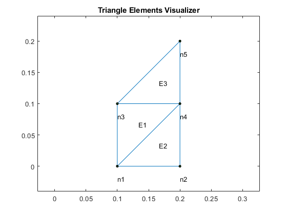
Define Geometry: node coordinates and elements

clear all;
nodes=[
    0.1,0;
    0.2,0;
    0.1,0.1;
    0.2,0.1;
    0.2,0.2;
    ];
elem=[4,3,1;
      1,2,4;
      3,4,5;
      ];
numNod=size(nodes,1);
numElem=size(elem,1);
numbering=1; %=1 shows the numbers for nodes and elements
plotElements(nodes,elem,numbering);

Define Coefficients vector of the model equation

In this case we use the Poisson coefficients defined in the problem above

a11=1;
a12=0;
a21=a12;
a22=a11;
a00=0;
f=0;
coeff=[a11,a12,a21,a22,a00,f];

Compute the global stiff matrix

Use the linearTriangElement function to compute the system by element

K=zeros(numNod);   %global Stiff Matrix
F=zeros(numNod,1); %global internal forces vector
Q=zeros(numNod,1); %global secondary variables vector
for e=1:numElem
  % compute element system
    [Ke,Fe]=linearTriangElement(coeff,nodes,elem,e);
  %
  % Assemble the elements
  %
    rows=[elem(e,1); elem(e,2); elem(e,3)];
    colums= rows;
    K(rows,colums)=K(rows,colums)+Ke; %assembly
    if (coeff(6) ~= 0)
        F(rows)=F(rows)+Fe;
    end
end % end for elements
% we save a copy of the initial F array
% for the postprocess step
Fini=F;
Kini=K;

Boundary Conditions (BC)

Impose Boundary Conditions for this example. In this case both essential and convection BC are considered.

fixedNodes=[1,3]; %Fixed Nodes (global num.)
freeNodes = setdiff(1:numNod,fixedNodes); %Complementary of fixed nodes

% ------------ Convection BC
convecNodes=[2,4,5];
beta=20; %Convection Coefficient
Tinf=30; %Bulk temperature
[K,Q]=applyConvTriang(convecNodes,beta,Tinf,K,Q,nodes,elem);

% ------------ Essential BC
u=zeros(numNod,1); %initialize u vector
u(fixedNodes)=100; %all of them are equal
F=F-K(:,fixedNodes)*u(fixedNodes);%here u can be different from zero only for fixed nodes

% modify the linear system, this is only valid if BC = 0.
Km=K(freeNodes,freeNodes);
Im=F(freeNodes)+Q(freeNodes);

Compute the solution

solve the System

format short e; %just to a better view of the numbers
um=Km\Im;
u(freeNodes)=um;
u'

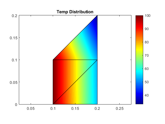
ans =

   1.0000e+02   5.3232e+01   1.0000e+02   5.2321e+01   3.3189e+01

Post Process

titol='Temp Distribution';
colorScale='jet';
plotContourSolution(nodes,elem,u,titol,colorScale)

Apply Convection Boundary Conditions on a Triangle mesh

We have implemented a small function to detect when a triangle has an edge of convection and apply the defined conditions.

function [K,Q]=applyConvTriang(indCV,beta,Tinf,K,Q,nodes,elem)
%------------------------------------------------------------------------
% (c) Numerical Factory 2018
%
% Apply a convection BC on a boundary of a triangulated domain.
%
% Input:
% indCV -> List of nodes on the convection boundary. They can be
%          non-connected but it needs:
%          i) Each connected component contains at least two nodes
%          ii) No corners are accepted (two edges of the same triangle).
%          If an unique triangle is a corner of the CV bondary, we have two call twice
%          this function (one time with each edge) and sume contributions
%
%          *           *
%          | \         |
%          |  \    =   |   +
%          *---*       *     *---*
%
% beta -> convection coefficient
% Tinf -> bulk temperature
% K    -> Global stiffness Matrix
% Q    -> Global Secondary variables Vector
% nodes-> all nodes (matrix of size nunNodx2)
% elem -> all elements (matrix of size numElemx3)
%
%------------------------------------------------------------------------
% Output:
% K -> Modified stiffness Matrix with the convection terms Kc on exit
%       K(indCV,indCV)=K(indCV,indCV)+Kc;
% Q -> The same for Q
%       Q(indCV)=Q(indCV)+Qc;
%
%------------------------------------------------------------------------
numElem=size(elem,1);
numCov=size(indCV,2);
if numCov==1
	error('applyConvTriang: Not unic node allow');
end
Kc=zeros(numCov,numCov);
Qc=zeros(numCov,1);
Kaux=(beta/6)*[2 1; 1 2];
Faux=0.5*beta*Tinf*[1; 1];
for k=1:numElem
  aux=[0,0,0]; %initial values (no node is found)
  for inod=1:3 %loop for the three nodes
      r=find(indCV==elem(k,inod)); %find if one node of element k is in the convection node list
      if(~isempty(r))
          aux(inod)=1; %put 1 on the local position found
      end
  end
    %
    % Now the aux vector is one of the following possibilities
    % aux=[0,0,0]  -> this element does not contain any convection node
    % aux=[1,0,0], [0,1,0], [0,0,1] -> contains only one convection node
    % aux=[1,1,0], [1,0,1], [0,1,1] -> contains two convection nodes
    % To classify which is the edge in local numbering, we consider aux as
    % a binary number expressed as power of 2: aux(1)*2^0+aux(2)*2^1+aux(3)*2^2
    % only 3 (first edge), 5 (third edge) or 6 (second edge)
    % are significant.
  number = aux(1)+2*aux(2)+4*aux(3);
  switch (number) %identify the appropriate edge
      case 3
          ij=[1,2];
      case 5
          ij=[3,1];
      case 6
          ij=[2,3];
      case 7
          error('applyConvTriang: Corners not allowed !!!!\n');
      otherwise, ij=[0,0];
  end
  if ( ij(1) > 0) %it's an existing edge
   n1=elem(k,ij(1));
   n2=elem(k,ij(2));
   h=norm(nodes(n1,:)-nodes(n2,:));
   fico=[find(indCV==n1), find(indCV==n2)];
   Kc(fico,fico)=Kc(fico,fico)+h*Kaux; %stiffness convection matrix
   Qc(fico)=Qc(fico)+h*Faux;           %convection vector
  end
end
K(indCV,indCV)=K(indCV,indCV)+Kc;
Q(indCV)=Q(indCV)+Qc;
end

(c)Numerical Factory 2017