FEM2D Fluids: Stream Lines using Triangular Elements

Consider the 2D equation model, a second order PDE equation with general coefficients a11, a12, a21, a22, a00, f :

Contents

State the problem: Equations for stream fluid problems (Poisson's Eq)

Model equations with 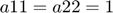and .

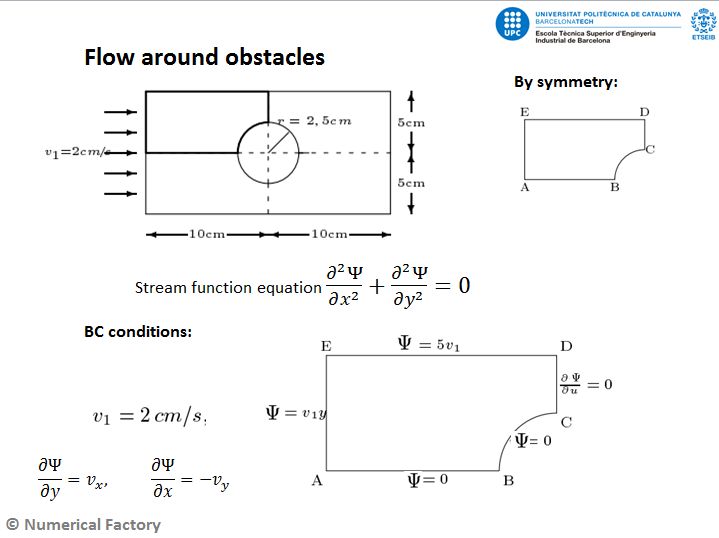
Load Geometry: node coordinates and elements

clear all;
eval('fluidMesh1'); % mesh on [0,2]x[0,1]
nodes=nodes*5; %escale to the size of the example [0,10]x[0,5]
numNod=size(nodes,1)
numElem=size(elem,1)
numbering=0; %=1 show the node and element numbers
plotElements(nodes,elem,numbering);
hold on;

numNod =

   325


numElem =

   579

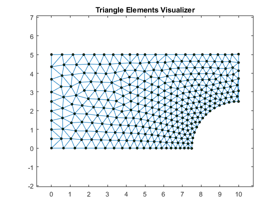
Select Boundary points

Hint: It depends on the domain geometry

indTop=find(nodes(:,2)> 4.99);
indBot=find(nodes(:,2)< 0.01);
indLeft=find(nodes(:,1)< 0.01);
indRigth=find(nodes(:,1)> 9.99);
indCircle=find(sqrt((nodes(:,1)-10).^2+nodes(:,2).^2)<2.501);
plot(nodes(indTop,1),nodes(indTop,2),'mo');
plot(nodes(indBot,1),nodes(indBot,2),'mo');
plot(nodes(indLeft,1),nodes(indLeft,2),'mo');
plot(nodes(indRigth,1),nodes(indRigth,2),'mo');
plot(nodes(indCircle,1),nodes(indCircle,2),'yd');
hold off;

Define Coefficients vector of the model equation

In this case we use the Poisson coefficients defined in the problem above

a11=1;
a12=0;
a21=a12;
a22=a11;
a00=0;
f=0;
coeff=[a11,a12,a21,a22,a00,f];

Compute the global stiff matrix

Use the linearTriangElement function to compute the system by element

K=zeros(numNod);   %global Stiff Matrix
F=zeros(numNod,1); %global internal forces vector
Q=zeros(numNod,1); %global secondary variables vector
for e=1:numElem
  % compute element system
    [Ke,Fe]=linearTriangElement(coeff,nodes,elem,e);
  %
  % Assemble the elements
  %
    rows=[elem(e,1); elem(e,2); elem(e,3)];
    colums= rows;
    K(rows,colums)=K(rows,colums)+Ke; %assembly
    if (coeff(6) ~= 0)
        F(rows)=F(rows)+Fe;
    end
end % end for elements
% we save a copy of the initial F array
% for the postprocess step
Fini=F;

Boundary Conditions (BC)

Impose Boundary Conditions for this example. In this case only essential and natural BC are considered. We will do a thermal example for convection BC (mixed).

fixedNodes=[indTop', indBot', indLeft', indCircle']; %Fixed Nodes (global num.)
freeNodes = setdiff(1:numNod,fixedNodes); %Complementary of fixed nodes
% ------------ Essential BC
inVel=2;
u=zeros(numNod,1); %initialize u vector
u(indTop)=5*inVel; %all of them are zero
u(indBot)=0; %all of them are zero
u(indCircle)=0; %all of them are zero
u(indLeft)=nodes(indLeft,2)*inVel;
F=F-K(:,fixedNodes)*u(fixedNodes);%here u can be different from zero only for fixed nodes
% ------------ Natural BC
Q(freeNodes)=0; %all of them are zero
% modify the linear system, this is only valid if BC = 0.
Km=K(freeNodes,freeNodes);
Im=F(freeNodes)+Q(freeNodes);

Compute the solution

solve the System

format short e; %just to a better view of the numbers
um=Km\Im;
u(freeNodes)=um;

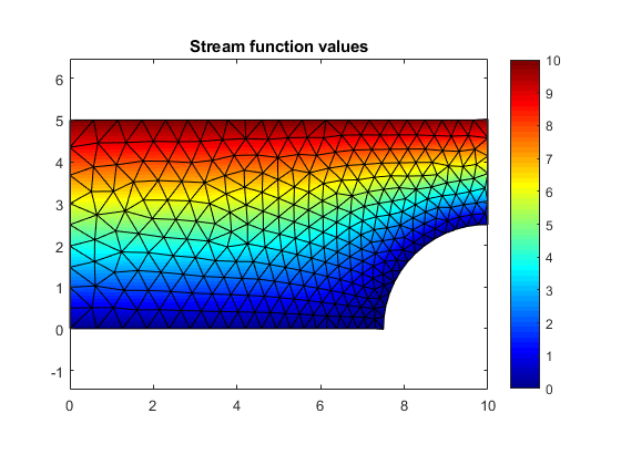
PostProcess: Compute secondary variables and plot results

Q=K*u-Fini;
titol='Stream function values';
colorScale='jet';
plotContourSolution(nodes,elem,u,titol,colorScale);

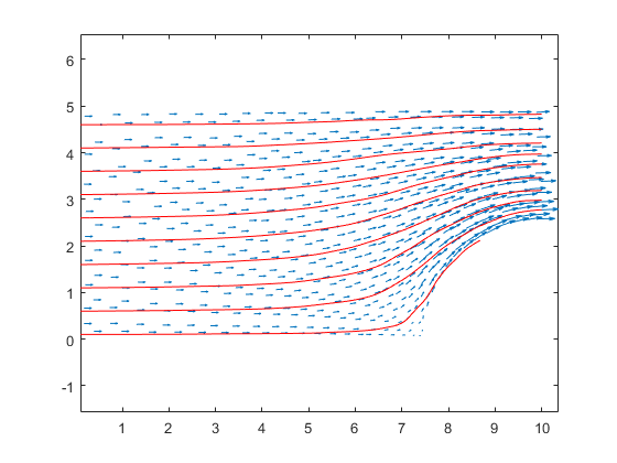
Stream lines

plotVelocityStream(nodes,elem,u)

Computing streamlines . . .

Exercise 1:

Compute the velocity at point p=[9,3] using the three mesh files: fluidMesh1,2,3. Compare the obtained results.

Hint: Using triangular meshes, velocities are constant in each element. They can be computed from the formula on T4-FEM2D-Applications pg. 25.

Sol:

fluidMesh1: elem= 161, vx = 3.7487e+00, vy = 1.0133e+00

fluidMesh2: elem= 225, vx = 3.8646e+00, vy = 1.0038e+00

fluidMesh3: elem= 233, vx = 3.9316e+00, vy = 1.0706e+00

(c)Numerical Factory 2017

Published with MATLAB® R2017b