FEM2D: Linear Quadrilateral Elements

Consider the 2D equation model, a second order PDE equation with general coefficients a11, a12, a21, a22, a00, f :

We will implement a Matlab function that computes the system of equations for a general linear quadrilateral element. This needs to implement the numerical integration of all the products of the shape functions (and their derivatives, see the formulas below.

Contents

For Linear Quadrilateral Elements we know that the formulas are not explicit and they have to be computed numerically. Here we will need the Gauss numerical quadrature function for quadrilaterals implemented in one of the previous practices. Explicitely we need the function files: gaussValues1D, gaussValues2DQuad, baryCoordQuad.

We remenber the formulas for this case:

Define Geometry: node coordinates and elements

eval('mesh2x2Quad');
numNod=size(nodes,1);
numElem=size(elem,1);
numbering=1;
figure()
plotElements(nodes,elem,numbering);

Define Coefficient vector of the model equation

In this case we use all constant coefficients equal to 1 for the model equation 2D.

a11=1;
a12=1;
a21=a12;
a22=a11;
a00=1;
f=1;
coeff=[a11,a12,a21,a22,a00,f];
K=zeros(numNod);
F=zeros(numNod,1);
for e=1:numElem
    %
    %Numerical evaluation of the integrals (Gauss N=2)
    %
    N=2; %number of GaussPoints
    [w,ptGaussRef]=gaussValues2DQuad(N);
    %
    % First compute Ke, Fe for each element
    %
    v1=nodes(elem(e,1),:);
    v2=nodes(elem(e,2),:);
    v3=nodes(elem(e,3),:);
    v4=nodes(elem(e,4),:);
    vertices=[v1;v2;v3;v4];
    % Shape functions
    Psi1=@(x,y)(1-x).*(1-y)/4;
    Psi2=@(x,y)(1+x).*(1-y)/4;
    Psi3=@(x,y)(1+x).*(1+y)/4;
    Psi4=@(x,y)(1-x).*(1+y)/4;
    shapeFunctions = @(x,y)[Psi1(x,y),Psi2(x,y),Psi3(x,y),Psi4(x,y)];
    % Shape function derivatives
    dPsi11=@(x,y) -(1-y)/4;
    dPsi21=@(x,y) (1-y)/4;
    dPsi31=@(x,y) (1+y)/4;
    dPsi41=@(x,y) -(1+y)/4;
    dPsi12=@(x,y) -(1-x)/4;
    dPsi22=@(x,y) -(1+x)/4;
    dPsi32=@(x,y) (1+x)/4;
    dPsi42=@(x,y) (1-x)/4;
    % Derivative matrix 2x4
    Jacob =@(x,y) [dPsi11(x,y), dPsi21(x,y),dPsi31(x,y),dPsi41(x,y);...
                   dPsi12(x,y), dPsi22(x,y),dPsi32(x,y),dPsi42(x,y)];

    % Compute the corresponding Gaussian points on the domain
    % evaluate Shape functions on Gaussian reference points
    xx = ptGaussRef(:,1);
    yy = ptGaussRef(:,2);
    evalPsi1 = Psi1(xx,yy);
    evalPsi2 = Psi2(xx,yy);
    evalPsi3 = Psi3(xx,yy);
    evalPsi4 = Psi4(xx,yy);
    % Evaluate Jacobian contribution for each point.
    % We use a Matlab cell variable in order to load each matrix.
    numPtG=size(xx,1);
    for i=1:numPtG
        Jtilde{i}=inv(Jacob(xx(i),yy(i))*vertices);
        evalDetJacob(i) = abs(det(Jacob(xx(i),yy(i))*vertices));
        Jacobian{i}=Jacob(xx(i),yy(i)); %derivatives of the shape functions
        shapeFun{i}=shapeFunctions(xx(i),yy(i));
    end
    %
    % element stiff matrix
    %
    Ke=zeros(4);
    Fe=zeros(4,1);
    if (coeff(1) ~= 0) %a11
        ik1=1; ik2=1; %index of the shape functions
        K11=zeros(4);
        for i=1:4  %Gauss integration
            for j=1:4
                suma=0;
                for ptG=1:numPtG
                    first=Jacobian{ptG}(1,i)*Jtilde{ptG}(ik1,1)+Jacobian{ptG}(2,i)*Jtilde{ptG}(ik1,2);
                    second=Jacobian{ptG}(1,j)*Jtilde{ptG}(ik2,1)+Jacobian{ptG}(2,j)*Jtilde{ptG}(ik2,2);
                    suma=suma+w(ptG)*first*second*evalDetJacob(ptG);
                end
                K11(i,j)=suma;
            end
        end
        Ke=Ke+coeff(1)*K11;
    end
    if (coeff(2) ~= 0) %a12
        ik1=1; ik2=2; %index of the shape functions
        K12=zeros(4);
        for i=1:4  %Gauss integration
            for j=1:4
                suma=0;
                for ptG=1:numPtG
                    first=Jacobian{ptG}(1,i)*Jtilde{ptG}(ik1,1)+Jacobian{ptG}(2,i)*Jtilde{ptG}(ik1,2);
                    second=Jacobian{ptG}(1,j)*Jtilde{ptG}(ik2,1)+Jacobian{ptG}(2,j)*Jtilde{ptG}(ik2,2);
                    suma=suma+w(ptG)*first*second*evalDetJacob(ptG);
                end
                K12(i,j)=suma;
            end
        end
        Ke=Ke+coeff(2)*K12;
    end
    if (coeff(3) ~= 0) %a21
        K21=K12'; %assuming isotropic values
        Ke=Ke+coeff(3)*K21;
    end
    if (coeff(4) ~= 0) %a22
        ik1=2; ik2=2; %index of the shape functions
        K22=zeros(4);
        for i=1:4  %Gauss integration
            for j=1:4
                suma=0;
                for ptG=1:numPtG
                    first=Jacobian{ptG}(1,i)*Jtilde{ptG}(ik1,1)+Jacobian{ptG}(2,i)*Jtilde{ptG}(ik1,2);
                    second=Jacobian{ptG}(1,j)*Jtilde{ptG}(ik2,1)+Jacobian{ptG}(2,j)*Jtilde{ptG}(ik2,2);
                    suma=suma+w(ptG)*first*second*evalDetJacob(ptG);
                end
                K22(i,j)=suma;
            end
        end
        Ke=Ke+coeff(4)*K22;
    end

    if (coeff(5) ~= 0) %a00
        K00=zeros(4);
        for i=1:4  %Gauss integration for the product of the shape functions
            for j=1:4
                suma=0;
                for ptG=1:numPtG
                    first=shapeFun{ptG}(i);
                    second=shapeFun{ptG}(j);
                    suma=suma+w(ptG)*first*second*evalDetJacob(ptG);
                end
                K00(i,j)=suma;
            end
        end
        Ke=Ke+coeff(5)*K00;
    end
    if (coeff(6) ~= 0) %f
        f=zeros(4,1);
        for i=1:4 %Gauss integration of the product f·ShapeFunt
            suma=0;
            for ptG=1:numPtG
                first=shapeFun{ptG}(i);
                suma=suma+w(ptG)*first*evalDetJacob(ptG);
            end
            f(i,1)=suma;
        end

        Fe=coeff(6)*f;
    end

  %
  % Assemble the elements
  %
    rows=[elem(e,1); elem(e,2); elem(e,3); elem(e,4)];
    colums= rows;
    K(rows,colums)=K(rows,colums)+Ke; %assembly
    if (coeff(6) ~= 0)
        F(rows)=F(rows)+Fe;
    end
end  %for elements

Boundary Conditions (BC)

Impose Boundary Conditions for this example. In this case only essential and natural BC are considered. We will do a thermal example for convection BC (mixed).

indRigth=[3;6;9];
indLeft=[1;4;7];
fixedNodes=[indLeft',indRigth']; %Fixed Nodes (global num.)
freeNodes = setdiff(1:numNod,fixedNodes); %Complementary of fixed nodes
% ------------ Essential BC
u=zeros(numNod,1); %initialize uu vector
u(indRigth)=0; %all of them are zero
u(indLeft)=0;
Fini=F; %copy of the original vector F
F=F-K(:,fixedNodes)*u(fixedNodes);%here u can be different from zero only for fixed nodes
% ------------ Natural BC
Q=zeros(numNod,1); %initialize Q vector
Q(freeNodes)=0; %all of them are zero
% modify the linear system, this is only valid if BC = 0.
Km=K(freeNodes,freeNodes);
Im=F(freeNodes)+Q(freeNodes);

Compute the solution

solve the System

format short e; %just to a better view of the numbers
um=Km\Im;
u(freeNodes)=um;
u

u =

            0
   1.1538e-01
            0
            0
   1.1538e-01
            0
            0
   1.1538e-01
            0

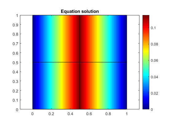
PostProcess: Compute secondary variables and plot results

Q=K*u-Fini
titol='Equation solution';
colorScale='jet';
plotContourSolution(nodes,elem,u,titol,colorScale)

Q =

  -1.7548e-01
            0
  -6.0096e-02
  -2.3558e-01
   2.7756e-17
  -2.3558e-01
  -6.0096e-02
  -2.7756e-17
  -1.7548e-01

Exercise 1:

For quadrilateral elements, implement a Matlab function that returns the element stiff matrix, Ke, and the Fe vector for each element depending on the coeff vector for the model equation.

function [Ke,Fe]=bilinearQuadElement(coeff,nodes,elem,e)

coeff --> coefficient vector = [a11,a12,a21,a22,a00,f] for the model equation

nodes --> matrix with the coordinates of the nodes

elem --> connectivity matrix defining the elements

e --> number of the present element

Exercise 2:

Consider now a thermal distribution problem of a square made with some material with conductivity coefficient and BC: . Compute the temperature at point using now the files mesh4x4Quad and mesh8x8Quad

Solution 4x4: t(p) = 4.0200e+01

Solution 8x8: t(p) = 4.0200e+01

(c)Numerical Factory 2019

Published with MATLAB® R2018a