FEM2D: Thermal convection problems using Quadrilateral Elements

Consider the 2D equation model, a second order PDE equation with general coefficients a11, a12, a21, a22, a00, f :

Equations for Thermal problems
State the problem:
Load Geometry: node coordinates and elements
Select Boundary points
Define Coefficients vector of the model equation
Compute the global stiff matrix
Boundary Conditions (BC)
Compute the solution
PostProcess: Compute secondary variables and plot results
Apply Convection Boundary Conditions
Exercise 1:

Equations for Thermal problems

Assume the case $$k_c=1$ and $$f=0$ .

State the problem:

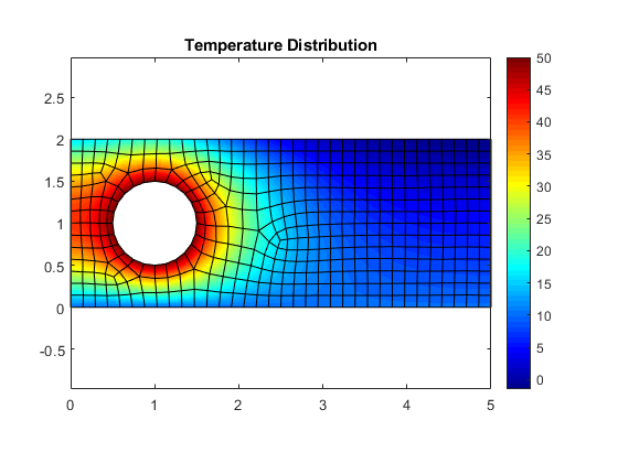
Consider the domain defined by mesh file meshPlacaForatQuad.m) ñ As a BC, consider the circle points at 50ºC and bottom boundary at 10ºC. Moreover, assume top boundary has convection with beta=2, and Tinf=-5ºC.

Load Geometry: node coordinates and elements

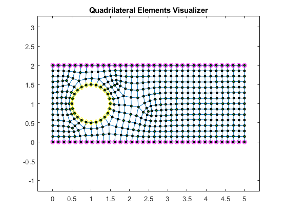
clear all;
close all;
eval('meshPlacaForatQuad');
numNod=size(nodes,1)
numElem=size(elem,1)
numbering=0;
plotElements(nodes,elem,numbering);

numNod =

   493


numElem =

   433

Select Boundary points

indTop=find(nodes(:,2)> 1.99);
indBot=find(nodes(:,2)< 0.01);
indCircle=find(sqrt((nodes(:,1)-1).^2+(nodes(:,2)-1).^2)<0.501);
hold on;
plot(nodes(indTop,1),nodes(indTop,2),'mo');
plot(nodes(indBot,1),nodes(indBot,2),'mo');
plot(nodes(indCircle,1),nodes(indCircle,2),'yd');
hold off;

Define Coefficients vector of the model equation

In this case we use the Poisson coefficients defined in the problem above

a11=1;
a12=0;
a21=a12;
a22=a11;
a00=0;
f=0;
coeff=[a11,a12,a21,a22,a00,f];

Compute the global stiff matrix

Use the linearTriangElement function to compute the system by element

K=zeros(numNod);   %global Stiff Matrix
F=zeros(numNod,1); %global internal forces vector
Q=zeros(numNod,1); %global secondary variables vector
for e=1:numElem
  % compute element system
  % Element stiffness Matrix
    [Ke,Fe]=bilinearQuadElement(coeff,nodes,elem,e);
  %
  % Assemble the elements
  %
    rows=[elem(e,1); elem(e,2); elem(e,3); elem(e,4)];
    colums= rows;
    K(rows,colums)=K(rows,colums)+Ke; %assembly
    if (coeff(6) ~= 0)
        F(rows)=F(rows)+Fe;
    end
end % end for elements
% we save a copy of the initial F array
% for the postprocess step
Kini=K;
Fini=F;

Boundary Conditions (BC)

Impose Boundary Conditions for this example. In this case only essential and natural BC are considered. We will do a thermal example for convection BC (mixed).

fixedNodes=[indBot', indCircle']; %Fixed Nodes (global num.)
freeNodes = setdiff(1:numNod,fixedNodes); %Complementary of fixed nodes

% ------------ Convection BC
convecNodes=indTop';
beta=2; %Convection Coefficient
Tinf=-5; %Bulk temperature
[K,Q]=applyConvQuad(convecNodes,beta,Tinf,K,Q,nodes,elem);

% ------------ Essential BC
u=zeros(numNod,1); %initialize u vector
u(indBot)=10; %all of them are zero
u(indCircle)=50; %all of them are zero
F=F-K(:,fixedNodes)*u(fixedNodes);%here u can be different from zero only for fixed nodes

% modify the linear system.
Km=K(freeNodes,freeNodes);
Im=F(freeNodes)+Q(freeNodes);

Compute the solution

solve the System

format short e; %just to a better view of the numbers
um=Km\Im;
u(freeNodes)=um;

PostProcess: Compute secondary variables and plot results

titol='Temperature Distribution';
colorScale='jet';
plotContourSolution(nodes,elem,u,titol,colorScale);

Apply Convection Boundary Conditions

function [K,Q]=applyConvQuad(indCV,beta,Tinf,K,Q,nodes,elem)
%
% (c) Numerical Factory 2018
%
%------------------------------------------------------------------------
% Apply a convection BC on a boundary of a quadrilateral meshed domain.
%
% Input:
% indCV -> List of nodes on the convection boundary. They can be
%          non-connected but it needs:
%          i) Each connected component contains at least two nodes
%          ii) Only one corner of a quadrilateral is accepted (two edges of the same quadrilateral).
%          If an unique quadrilateral is part of the CV bondary, we have two call twice
%          this function: one time with a corner and then the rest, and sume contributions
%
%   *      *           *                *          *              *
%   |      |           |                |          |              |
%   |      |     =     |          +     |   o be   |    +         |
%   *------*           *------*       ..*          *..     *------*
%
%
%  Hint: See the Triang version for the rest of variables and more explanations
%------------------------------------------------------------------------------

numElem=size(elem,1);
numCo=size(indCV,2);
if (numCo==1)
    error('applyConvQuad: It can''t manage a single node');
end
Kaux=(beta/6)*[2 1; 1 2];
Faux=0.5*beta*Tinf*[1; 1];
for k=1:numElem
  aux=[0,0,0,0];
  for j=1:4
    r=find(indCV==elem(k,j)); %find if j node of element k is in the convection nodes list
      if(~isempty(r)), aux(j)=1; end
  end
  %See the Triang version for the explanation of the binary number
  number=aux*[1;2;4;8];
  % Here we codify both edges and corners on the boundaries
  switch (number)
    case  3, ij=[1,2,0,0];  % edge 1:   aux=[1,1,0,0];
    case  6, ij=[2,3,0,0];  % edge 2:   aux=[0,1,1,0];
    case  7, ij=[1,2,2,3];  % corner 2: aux=[1,1,1,0];
    case  9, ij=[4,1,0,0];  % edge 4
    case 11, ij=[4,1,1,2];  % corner 1
    case 12, ij=[3,4,0,0];  % edge 3
    case 13, ij=[3,4,4,1];  % corner 4
    case 14, ij=[2,3,3,4];  % corner 3
    case 15, error('applyConvQuad: It can''t manage two corners'); % two corners
    otherwise, ij=[0,0,0,0];
  end
  for j=1:2:3
   if ~ij(j)==0
    n1=elem(k,ij(j));
    n2=elem(k,ij(j+1));
    h=norm(nodes(n1,:)-nodes(n2,:));
    fico=[n1, n2];
    K(fico,fico)=K(fico,fico)+h*Kaux;
    Q(fico)=Q(fico)+h*Faux;
   end
  end
end
end %function

Exercise 1:

Compute the temperature for point p=[1.5, 1.2].

Sol: pElem = 248, nodes=[288, 106, 105, 287], tempP = 4.7120e+01

(c)Numerical Factory 2018